About the Project
When I started knowing more about Deep Learning and had gone through sufficient number of blog posts stating their own learning paths for this specific area, a man called Jeremy Howard popped up quite a number of times and how he and Rachel Thomas made a practical DL course using their own library, FastAI. Now, many of the readers here would have suggested me otherwise as many of the blog posts did, to start (obviously) with Andrew Ng’s deeplearning.ai specialization. But being a more getting-my-hands-dirty-and-learning-on-the-field type of person, I chose the former to start with. Do not get me wrong, I will soon be shifting to Ng’s Coursera specialization, almost the Bible of DL at present. But, FastAI is something, and which I liked the most, that does not go into nitty-gritties of things, but will provide you with the best possible result.
This is my first project based on Convolutional Neural Networks using FastAI and predicts the type of art when inputted with an image, whether it is a painting, a drawing, a sculpture, an iconography or an engraving.
Project Details
- The Kaggle notebook for this project to fork is linked here.
- The dataset for 5000 images divided into 5 categories is taken from a Kaggle source.
- The Github repo for this can be accessed from here.
- Python libraries used extensively are :
Learning and Prediction
Disclaimer: There are some steps below which are Kaggle specific only and will be mentioned as such beforehand.
A. Importing the libraries
Both Kaggle and Google Colab comes pre-installed with fastai and pytorch. But if you are doing this on your local computer for the first time, you have to download pytorch and fastai, in that order, preferably on a virtual environment like conda.
More on downloading Pytorch is available on their website.
After pytorch is installed, run conda install -c fastai fastai on a Linux terminal to get started with this project.
#Imports all the libraries used in the project
from fastai import *
from fastai.vision import *
B. Declaring PATH
Take PATH to be the parent folder of the training and validation set.
In Kaggle, this is the folder. If on local system, the PATH will be different.
PATH = "../input/art-images-drawings-painting-sculpture-engraving/art_dataset_cleaned/art_dataset"
C. Accessing the images and labels
If we take a look at the dataset, we will notice that the label names are actually the folders, i.e., all drawings are contained in a folder called drawings, all paintings in a folder called paintings and so on, in an ImageNet style. And also, the training and validation set have already been made by the dataset provider.
But before that, we have to declare how we are going to handle the image transforms. FastAI provides with a function called get_tranforms() within which we can mention how we transform the images, as here, we do not want our CNN to be trained on images which are flipped in any way. That means if a drawing is flipped or rotated in any way or to any degree, that image becomes a completely different picture and we do not want our CNN to learn that. Maybe in case of satellite images of land and sea, we can flip the images because then, the image does not become a totally different one.
tfms = get_transforms(do_flip=False)
#do_flip=False because of reason mentioned above.
data = ImageDataBunch.from_folder(PATH, train="training_set", valid="validation_set", ds_tfms=tfms, size=200, num_workers=0)
#We direct train and valid to the respective sets inside the folder.
Now we check the data whether it is loaded properly or not.
data.show_batch(rows=3, figsize=(5,5))
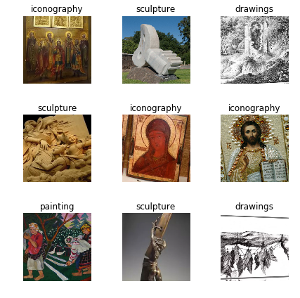
data.classes lists the classes or the labels of the images.
['drawings', 'engraving', 'iconography', 'painting', 'sculpture']
D. Downloading trained weights from Resnet34 or Resnet50
This is a Kaggle specific step. Since Kaggle kernels are read-only, so we add trained Resnet34 model to our kernel by selecting Add Data from the right hand section of the screen and we also make a directory for copying the .pth model to our filesystem.
cache_dir = os.path.expanduser(os.path.join('~','.torch'))
#First make a ~/.torch folder if not available.
if not os.path.exists(cache_dir):
    os.makedirs(cache_dir)
models_dir = os.path.join(cache_dir,'models')
#then make ~/.torch/models, if not already available.
if not os.path.exists(models_dir):
    os.makedirs(models_dir)
Then we copy the .pth folder to our filesystem.
!cp ../input/resnet34/resnet34.pth ~/.torch/models/resnet34-333f7ec4.pth
And we declare another PATH variable to be used in the CNN learner.
MODEL_PATH = '/tmp/models'
E. Training the CNN to learn from data
If you are not using Kaggle, ignore the whole section D and start again from this step.
So now, we declare our cnn_learner to be trained from data by taking training and validation images from PATH previously declared.
learn = cnn_learner(data, models.resnet34, metrics=accuracy, model_dir=MODEL_PATH)
#Ignore model_dir attribute if on local system. It is a Kaggle specific step again.
Now we use fit_one_cycle() and mention the no. of epochs we want it to train the first time.
learn.fit_one_cycle(4)
| epoch | train_loss | valid_loss | accuracy | time |
|---|---|---|---|---|
| 0 | 0.489632 | 0.265858 | 0.901869 | 02:02 |
| 1 | 0.301034 | 0.202761 | 0.925234 | 01:56 |
| 2 | 0.233835 | 0.189954 | 0.929907 | 01:57 |
| 3 | 0.199139 | 0.181202 | 0.934579 | 01:56 |
We can already see from the very first training trial, due to the Resnet34 weights, we have reached an accuracy of 93.4% just by altering the last few layers of the network.
But we will see the learning rates further and try to improve the model more. So we unfreeze() the model and train it again from the start with specified learning rates. To specifiy learning rates we first plot the loss v/s learning rate to infer from it.
#We save the model first for future use, if needed.
learn.save('stage-1')
learn.unfreeze()
learn.lr_find()
learn.recorder.plot()
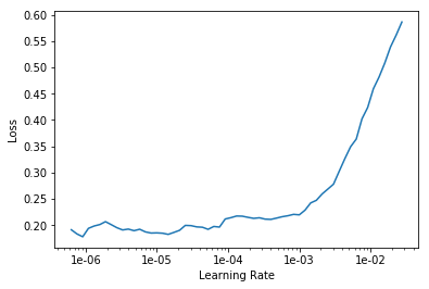
We can see from the above plot the when learning rate is around between 1e-05 to 1e-04, the loss is the minimum and rise to the peak from LR 1e-03. So we fit the learner again, now with 2 epochs.
learn.fit_one_cycle(2,max_lr=slice(1e-05,1e-04))
| epoch | train_loss | valid_loss | accuracy | time |
|---|---|---|---|---|
| 0 | 0.186892 | 0.163934 | 0.940421 | 02:01 |
| 1 | 0.139290 | 0.150968 | 0.940421 | 02:01 |
We have now achieved an accuracy of around 94%. Now we perform the process again and see if we can achieve a greater accuracy.
learn.save('stage-2')
learn.unfreeze()
learn.lr_find()
learn.recorder.plot()
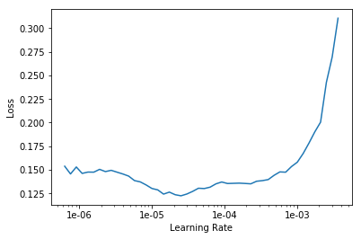
learn.fit_one_cycle(2,max_lr=slice(1e-06,1e-05))
| epoch | train_loss | valid_loss | accuracy | time |
|---|---|---|---|---|
| 0 | 0.114904 | 0.150118 | 0.947430 | 02:00 |
| 1 | 0.110616 | 0.144483 | 0.947430 | 02:00 |
learn.save('stage-3')
F. Testing externally inputted images for prediction
With an achieved accuracy of 94.7%, we now input our own images by declaring the PATHs to the images and test it on our learner, whether it predicts correct categories or not.
FastAI’s open_image() reads the image for you. Here, I have downloaded one image of each class from Google and test it on the learner.
#this is Kaggle specific. You can declare your own paths.
PRED_PATH = "../input/for-testing-art-images-cnn"
img_icono = open_image(f'{PRED_PATH}/icono.jpg')
img_drawing = open_image(f'{PRED_PATH}/drawing.jpg')
img_engraving = open_image(f'{PRED_PATH}/engraving.png')
img_painting = open_image(f'{PRED_PATH}/painting.jpg')
img_sculpt = open_image(f'{PRED_PATH}/sculpture.jpg')
Now we load the previous stage-3 and predict the classes for these images.
learn.load('stage-3')
pred_class = learn.predict(img_icono)
pred_class
Out: (Category iconography, tensor(2), tensor([6.4216e-07, 2.8668e-06, 9.9999e-01, 1.5303e-06, 2.8591e-08]))
pred_class = learn.predict(img_drawing)
pred_class
Out: (Category drawings, tensor(0), tensor([9.5027e-01, 3.9309e-02, 3.6643e-04, 3.6381e-03, 6.4128e-03]))
pred_class = learn.predict(img_painting)
pred_class
Out: (Category drawings, tensor(0), tensor([0.5862, 0.1606, 0.0067, 0.2367, 0.0097]))
pred_class = learn.predict(img_sculpt)
pred_class
Out: (Category sculpture, tensor(4), tensor([1.5215e-04, 1.6432e-04, 5.0656e-04, 2.4123e-04, 9.9894e-01]))
pred_class = learn.predict(img_engraving)
pred_class
Out: (Category engraving, tensor(1), tensor([4.5636e-02, 9.5435e-01, 1.0390e-05, 2.7635e-06, 4.8394e-06]))
Taking this project forward
I am satisfied with the accuracy I achieved via this CNN. The only wrong prediction it does is it tells a painting of Mona Lisa to be a drawing. I cannot blame it exactly as the picture seems to be a drawing to human eyes too (sometimes). But to clear this conclusion, I tested Van Gogh’s Starry Night (not shown above) and it correctly predicts it to be a painting.
What I can do more to make this more accessible is to make a web UI out of it and host it on my local PC or maybe rent a small EC2 instance on AWS or Heroku to make a sole web app out of this. But that is for another post, while I am still studying on how to deploy ML or DL models on the web the easiest way possible.